Polarplot in R
Polarplot
The polarplot presents directions and angles. There are several polarplot functions from different packages. In my oppinion, the polar.plot() function by Paul Murrell is the best option. As far as I know, it does not come with a package, but it's available on Paul's website.
Notice that as in all other circle functions all information must be given in radians instead of degrees! Thus, all degrees need to be transformed into radians (radians = angle * 2pi / 360). Moreover, the direction is counter-clockwise and starts at 3 o'clock or 90°, respectively. This can be adjusted using the arguments theta.clw = TRUE and theta.zero = pi/2. With default settings the polarplot looks like this:

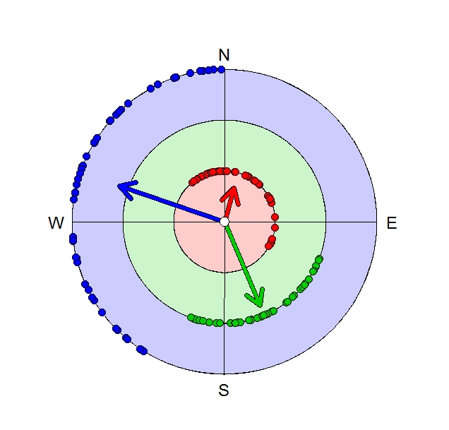
In some cases it might be useful to show the concentrations of points by vector arrows. These can be added to the existing polarplot using the arrows() function.
This graphic was created using the following code :
set.seed(610)
r1 <- runif(50, 210, 360) * pi/180
set.seed(610)
r2 <- runif(50, 110, 200) * pi/180
set.seed(610)
r3 <- c(runif(25, 320, 360), runif(25, 0, 120)) * pi/180


polar.plot(0, 0, theta.clw = TRUE, theta.zero = pi/2, dir = 4, points.cex = 0, text.lab = c("", "", "", ""), pi2.lab = FALSE, rlabel.method = 0,
   grid.circle.pos = 1:3)
polygon(3 * sin(seq(0, 2 * pi, len = 1000)), 3 * cos(seq(0, 2 * pi, len = 1000)), col = adjustcolor(4, 0.2))
polygon(2 * sin(seq(0, 2 * pi, len = 1000)), 2 * cos(seq(0, 2 * pi, len = 1000)), col = "white")
polygon(2 * sin(seq(0, 2 * pi, len = 1000)), 2 * cos(seq(0, 2 * pi, len = 1000)), col = adjustcolor(3, 0.2))
polygon(sin(seq(0, 2 * pi, len = 1000)), cos(seq(0, 2 * pi, len = 1000)), col = "white")
polygon(sin(seq(0, 2 * pi, len = 1000)), cos(seq(0, 2 * pi, len = 1000)), col=adjustcolor(2, 0.2))
polar.plot(3, r1, theta.clw = TRUE, theta.zero = pi/2, points.bg = 4, points.pch = 21, points.cex = 1.5, overlay = 2, dir = 4, text.lab = c("N", "E", "S", "W"),
   pi2.lab = FALSE, rlabel.method = 0, grid.circle.pos = 1:3)
polar.plot(2, r2, theta.clw = TRUE, theta.zero = pi/2, points.bg = 3, points.pch = 21, points.cex = 1.5, overlay = 1)
polar.plot(1, r3, theta.clw = TRUE, theta.zero = pi/2, points.bg = 2, points.pch = 21, points.cex = 1.5, overlay = 1)


t.md <- circ.summary(r1)[1,2]
t.mvl <- (circ.summary(r1)[1,3]) * 3
x2 <- t.mvl * sin(t.md)
y2 <- t.mvl * cos(t.md)
arrows(0, 0, x2, y2,length = 0.25, lwd = 7, col = 1)
arrows(0, 0, x2, y2,length = 0.25, lwd = 5, col = 4)

t.md <- circ.summary(r2)[1,2]
t.mvl <- (circ.summary(r2)[1,3]) * 2
x2 <- t.mvl * sin(t.md)
y2 <- t.mvl * cos(t.md)
arrows(0, 0, x2, y2, length = 0.25, lwd = 7, col = 1)
arrows(0, 0, x2, y2, length = 0.25, lwd = 5, col = 3)

t.md <- circ.summary(r3)[1,2]
t.mvl <- (circ.summary(r3)[1,3])
x2 <- t.mvl * sin(t.md)
y2 <- t.mvl * cos(t.md)
arrows(0, 0, x2, y2, length = 0.25, lwd = 7, col = 1)
arrows(0, 0, x2, y2, length = 0.25, lwd = 5, col = 2)

polar.plot(0, 0, points.bg = "white", points.pch = 21, points.cex = 2, overlay = 1)
Tags
Polarplot, angle diagram, directions, degrees to radians, vectors, different colors, colours, transparency, background colors, dependent size, dependent colors, x-axis, y-axis, bottom, left, top, right, labels, without ggplot