Polarplot in R erstellen
Polarplot
Der Polarplot dient zur Darstellung von Richtungs- und Winkeldaten. Es gibt diverse Polarplot-Funktionen aus unterschiedlichen Paketen. Mir persönlich gefällt die polar.plot()-Funktion von Paul Murrell am besten. Soweit ich weiß wird sie in keinem Paket geliefert, aber sie wird auf der Website von Paul zur Verfügung gestellt.
Zu beachten ist, dass wie bei den meisten Kreisfunktionen auch hier alle Angaben in Radiant statt in Winkelgrad zu machen sind! Daher müssen zur korrekten Darstellung alle Winkel in Radiant umgerechnet werden (Radiant = Winkel * 2pi / 360). Außerdem verläuft die Richtung entgegen des Uhrzeigersinns und startet bei 3 Uhr bzw. 90°. Dies kann aber über die Argumente theta.clw = TRUE und theta.zero = pi/2 ausgeglichen werden. Mit den Standardeinstellungen sieht der Polarplot so aus:

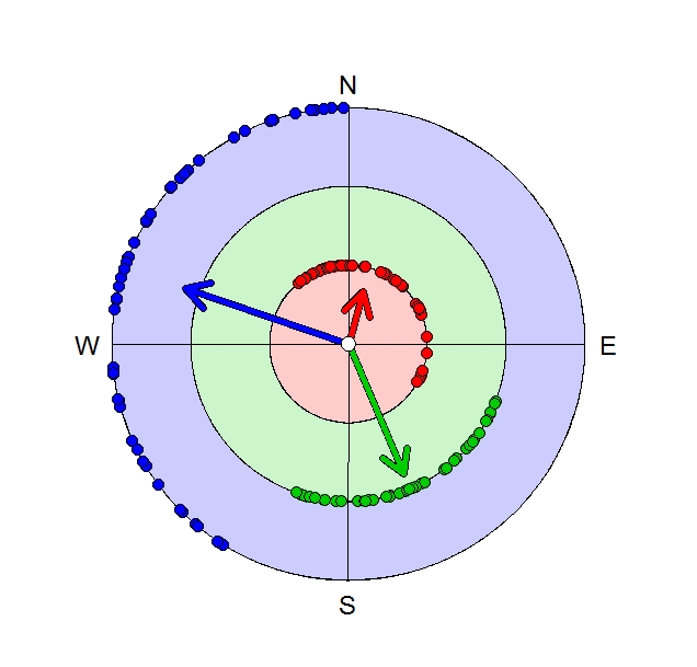
Häufig ist es sinnvoll, die Konzentration der Punkte z.B. mit Vektorpfeilen darzustellen. Diese lassen sich ganz einfach mithilfe der arrows()-Funktion zum bestehenden Polarplot hinzufügen.
Diese Grafik wurde mit folgendem Code erstellt:
set.seed(610)
r1 <- runif(50, 210, 360) * pi/180
set.seed(610)
r2 <- runif(50, 110, 200) * pi/180
set.seed(610)
r3 <- c(runif(25, 320, 360), runif(25, 0, 120)) * pi/180


polar.plot(0, 0, theta.clw = TRUE, theta.zero = pi/2, dir = 4, points.cex = 0, text.lab = c("", "", "", ""), pi2.lab = FALSE, rlabel.method = 0,
   grid.circle.pos = 1:3)
polygon(3 * sin(seq(0, 2 * pi, len = 1000)), 3 * cos(seq(0, 2 * pi, len = 1000)), col = adjustcolor(4, 0.2))
polygon(2 * sin(seq(0, 2 * pi, len = 1000)), 2 * cos(seq(0, 2 * pi, len = 1000)), col = "white")
polygon(2 * sin(seq(0, 2 * pi, len = 1000)), 2 * cos(seq(0, 2 * pi, len = 1000)), col = adjustcolor(3, 0.2))
polygon(sin(seq(0, 2 * pi, len = 1000)), cos(seq(0, 2 * pi, len = 1000)), col = "white")
polygon(sin(seq(0, 2 * pi, len = 1000)), cos(seq(0, 2 * pi, len = 1000)), col=adjustcolor(2, 0.2))
polar.plot(3, r1, theta.clw = TRUE, theta.zero = pi/2, points.bg = 4, points.pch = 21, points.cex = 1.5, overlay = 2, dir = 4, text.lab = c("N", "E", "S", "W"),
   pi2.lab = FALSE, rlabel.method = 0, grid.circle.pos = 1:3)
polar.plot(2, r2, theta.clw = TRUE, theta.zero = pi/2, points.bg = 3, points.pch = 21, points.cex = 1.5, overlay = 1)
polar.plot(1, r3, theta.clw = TRUE, theta.zero = pi/2, points.bg = 2, points.pch = 21, points.cex = 1.5, overlay = 1)


t.md <- circ.summary(r1)[1,2]
t.mvl <- (circ.summary(r1)[1,3]) * 3
x2 <- t.mvl * sin(t.md)
y2 <- t.mvl * cos(t.md)
arrows(0, 0, x2, y2,length = 0.25, lwd = 7, col = 1)
arrows(0, 0, x2, y2,length = 0.25, lwd = 5, col = 4)

t.md <- circ.summary(r2)[1,2]
t.mvl <- (circ.summary(r2)[1,3]) * 2
x2 <- t.mvl * sin(t.md)
y2 <- t.mvl * cos(t.md)
arrows(0, 0, x2, y2, length = 0.25, lwd = 7, col = 1)
arrows(0, 0, x2, y2, length = 0.25, lwd = 5, col = 3)

t.md <- circ.summary(r3)[1,2]
t.mvl <- (circ.summary(r3)[1,3])
x2 <- t.mvl * sin(t.md)
y2 <- t.mvl * cos(t.md)
arrows(0, 0, x2, y2, length = 0.25, lwd = 7, col = 1)
arrows(0, 0, x2, y2, length = 0.25, lwd = 5, col = 2)

polar.plot(0, 0, points.bg = "white", points.pch = 21, points.cex = 2, overlay = 1)